Add a header and the date for each of the columns (assignments) in the range.
Cell B2.
Text "Date".
Cell Range C2: S2
Text: "22-Aug, 29-Aug,…12-Dec"
Answer: Use the following steps to complete this task in explanation:
Explanation:
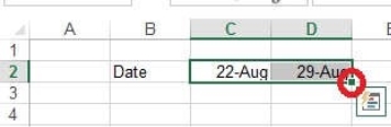
Step 1: Click Cell B2. Type the text: Date
Step 2: Click cell C2. Type the text: 22-Aug
Step 3: Click cell D2. Type the text: 29-Aug
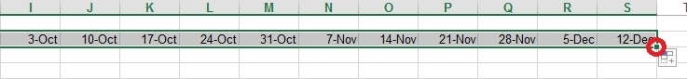
Step 3: Click cell C2, then shift-click cell D2.
Step 4: Copy until cell S2 (by dragging from cell D2 to cell S2).
Answer is in the explanation below.
Reference / correct answer:
See Explanation Below For Answer
Step 1: Click Cell B2. Type the text: Date
Step 2: Click cell C2. Type the text: 22-Aug
Step 3: Click cell D2. Type the text: 29-Aug
Step 3: Click cell C2, then shift-click cell D2.
Step 4: Copy until cell S2 (by dragging from cell D2 to cell S2).
Question 2
Apply a cell style
Cell range A2:S2
Style 40% - Accent3
Answer: Use the following steps to complete this task in explanation:
Explanation:
Step 1: Open the correct worksheet (Section 3 Worksheet).
Step 2: Click in cell A2.
Step 3: Press down the Shift key and click in cell S2.
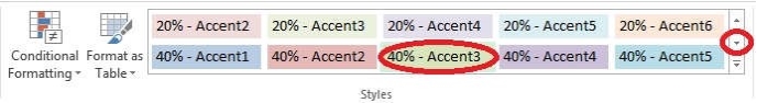
Step 4: On the Home tab, under Format, scroll down until you see 40% . Accent3, and click on it.
Answer is in the explanation below.
Reference / correct answer:
See Explanation Below For Answer
Step 1: Open the correct worksheet (Section 3 Worksheet).
Step 2: Click in cell A2.
Step 3: Press down the Shift key and click in cell S2.
Step 4: On the Home tab, under Format, scroll down until you see 40% . Accent3, and click on it.
Question 3
Add conditional formatting.
Color Scales: Green –White-Red Color Scale
Midpoint: Percentile, "70" Maximum: Number, "25"
Answer: Use the following steps to complete this task in explanation:
Explanation:
Step 1: Click cell C3
Step 2: Shift-Click cell S25.
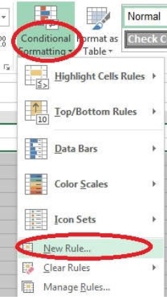
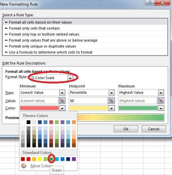
Step 3: On the Home tab, under Format, choose Conditional Formatting, and choose New Rule...
Step 4: In the New Formatting Rule dialog box set Format Style to: 3-Color Scale, and set Minimum Color to Green.
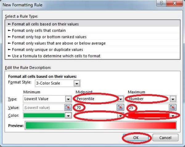
Step 5: In the same dialog box set Midpoint type to Percentile, set Midpoint Value to 70, and set Midpoint Color to White. Also set Maximum Type to Number, Maximum value to 25, and Maximum Color to Red. Finally click OK.
Answer is in the explanation below.
Reference / correct answer:
See Explanation Below For Answer
Step 1: Click cell C3
Step 2: Shift-Click cell S25.
Step 3: On the Home tab, under Format, choose Conditional Formatting, and choose New Rule...
Step 4: In the New Formatting Rule dialog box set Format Style to: 3-Color Scale, and set Minimum Color to Green.
Step 5: In the same dialog box set Midpoint type to Percentile, set Midpoint Value to 70, and set Midpoint Color to White. Also set Maximum Type to Number, Maximum value to 25, and Maximum Color to Red. Finally click OK.
Limited Time Offer – Save Now!
Don’t miss out — get full access at the best price.